Completed2026

RF Modulation Classifier with Real-Time C++ Inference

A 1D CNN trained on raw IQ samples to classify 24 radio modulation schemes, exported to ONNX and served from a C++ pipeline whose predictions are validated to exact parity with PyTorch.

92%

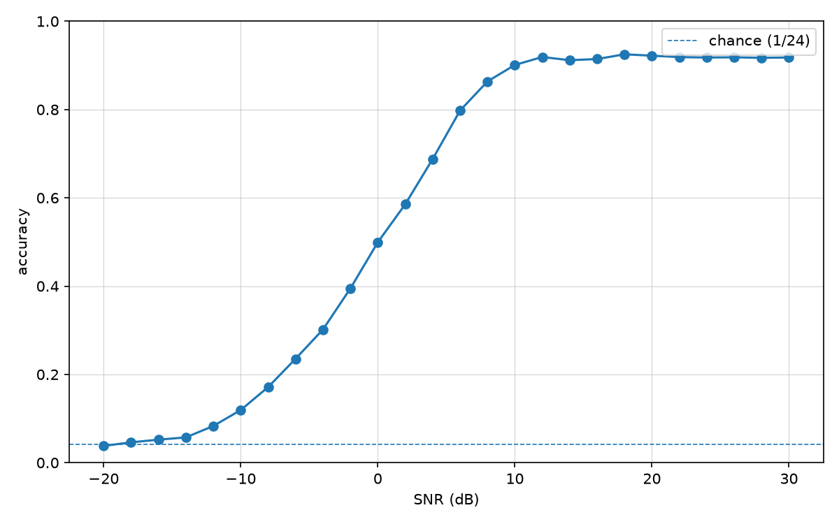
Accuracy above +10 dB SNR

1,290 inf/s

C++ throughput

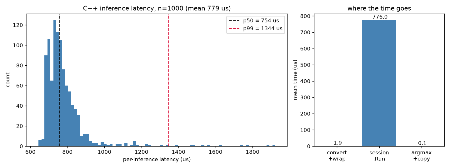
775 μs

Mean latency

1000 / 1000

PyTorch parity

The question

How quickly can a signal become useful information?

My interest in defense and trading technology led me here: the time between receiving a signal and acting on it can matter as much as the information itself. I wanted to explore one part of that chain—recognizing a radio signal’s modulation—and carry a machine-learning model into a measured C++ inference pipeline.

This project classifies recorded signals. It does not demonstrate a deployed defense system, a trading advantage, or an end-to-end radio link.

A little radio, before the code.

RF is the medium.

RF stands for radio frequency. Wireless systems use electromagnetic waves to carry information between transmitters and receivers. The receiver observes a mixture of the intended signal, noise, and effects of the channel.

Modulation is how we write on it.

A transmitter varies a carrier’s amplitude, frequency, or phase to represent information. PSK uses phase; QAM combines amplitude and phase. Identifying the modulation helps a receiver decide how to interpret an unfamiliar signal.

More possible symbols can carry more bits in each transmission interval, but closely spaced symbols become harder to distinguish in noise. That tradeoff makes signal quality essential context for any accuracy claim.

Background reading: PySDR’s digital modulation guide

See what noise takes away.

Explore a signal

Choose a modulation scheme, then lower the signal-to-noise ratio. Watch distinct symbols become harder to tell apart.

Modulation

Signal-to-noise ratio: 15 dB

More noiseCleaner signal

2 bits per symbol. Fewer symbols leave more space between possible messages.

Illustrative normalized symbols with synthetic Gaussian noise. Outlying points are clipped to the plot. This is not the trained classifier or its measured accuracy.

From samples to a decision.

Capture the shape

Raw in-phase (I) and quadrature (Q) samples retain the amplitude and phase structure of the signal.

Learn the patterns

A 1D convolutional network learns features across the samples and predicts one of 24 modulation classes.

Measure the runtime

Exporting to ONNX lets the C++ pipeline run the model, compare predictions, and profile inference latency.

What the measurements taught me.

The existing benchmark reports about 92% accuracy above +10 dB SNR, but performance falls toward chance in heavy noise. An accuracy-versus-SNR curve is therefore more informative than a single overall score.

The C++ pipeline reports 775 μs mean inference latency and 1,000 matching predictions against PyTorch. Prediction parity checks the export path; it does not establish accuracy on unseen real-world radio captures.

The surprising systems result: adding a producer/consumer thread did not help. Model execution already consumed 99.7% of inference time, so synchronization cost more than the small amount of work it could hide. The next useful experiments belong inside the inference workload: quantization, batching, or a smaller model.

Technologies

PyTorchONNX RuntimeC++CMake

Implementation details

—Trained a ~2.2M-parameter 1D CNN (four Conv1d → ReLU → MaxPool blocks) directly on raw IQ samples rather than spectrograms — magnitude spectrograms discard phase, and phase is exactly where PSK/QAM schemes encode information. Trained on the full RadioML 2018.01A dataset: 2.55M recordings, 24 modulation classes, −20 to +30 dB SNR.
—Reported accuracy as a curve over SNR rather than one aggregate number, since the aggregate (~55%) is close to meaningless without it: near chance below −15 dB, crossing 50% around 0 dB, and plateauing near 92% above +10 dB.
—Exported to ONNX Runtime and built a C++ inference pipeline validated to exact parity with PyTorch — 1000/1000 matching predictions — sustaining ~1,290 inferences/sec at 775 μs mean latency (1.7 ms p99) and 55 MB peak working set.
—Instrumented per-stage latency profiling: session.Run() alone accounts for 99.7% of inference time. Measured a two-thread producer/consumer pipelining variant as a follow-up — and reported it as a negative result: synchronization cost more than the ~1.4 μs of hideable work it was competing for, so it didn't help. The only real path to faster is inside the model (quantization, batching, a smaller head), not around it.

Results

Line chart of classification accuracy rising from near-chance at -20 dB SNR to about 92% above +10 dB — Accuracy as a function of SNR — the curve that actually matters, not the aggregate.

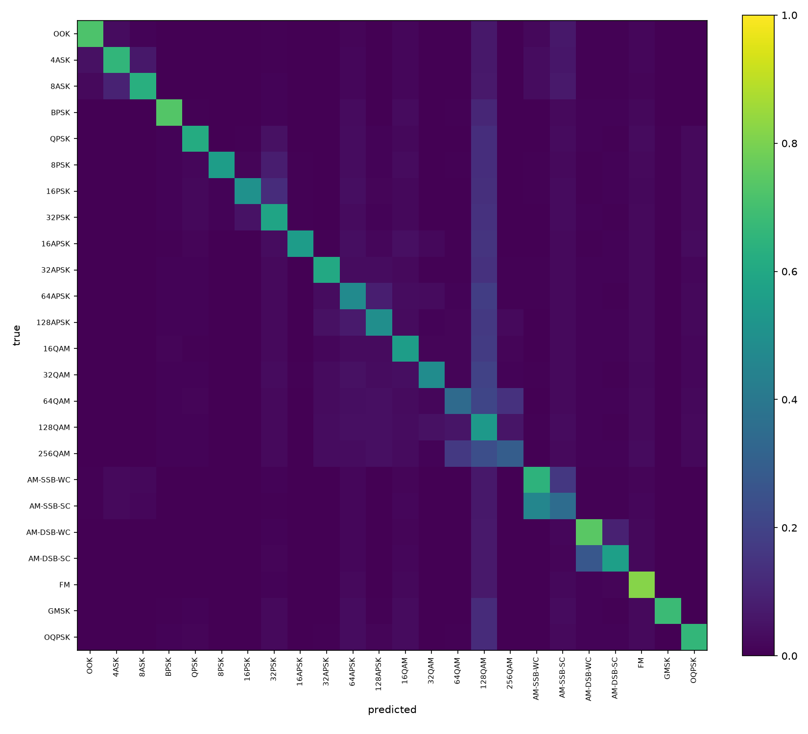
24x24 confusion matrix heatmap with a strong diagonal, showing where the model confuses adjacent QAM orders — Confusion matrix across all 24 classes — most error mass sits between adjacent QAM orders.

Histogram of C++ inference latency centered around 775 microseconds, plus a bar chart showing session.Run as 99.7% of time — 1,000-sample C++ latency distribution, and where the time actually goes per inference.

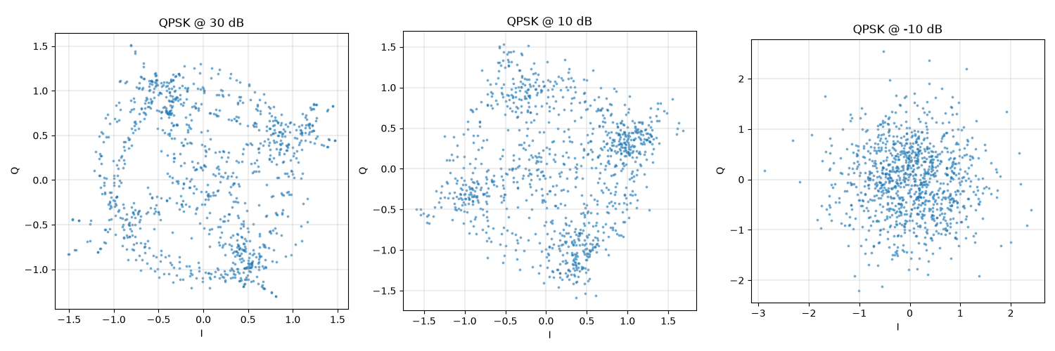
Three IQ constellation scatter plots of QPSK at 30dB, 10dB, and -10dB SNR, showing the clusters smearing into noise — QPSK constellation at 30, 10, and −10 dB — the same signal, dissolving into noise.